Flow, Vector Field and Tensor Field Visualization

Many phenomena in science cannot be represented adequately by a single value (or scalar). As soon as directional information becomes important, the data are represented as vectors or tensors. An example for this is the simulation of air in a closed room. While single values are enough to represent the temperature at every position in the room, vectors are required to represent the flow of the air in the room. This example also shows the strong connection between vector field and flow visualisation. Vector fields are usually the basis for flow visualisation applications.

In more complex cases – when not only a single direction but also a directional distribution is given – even a vector is not sufficient. In this case, tensors are used. Tensors are the generalisation of scalars and vectors. A scalar is a tensor of zeroth order and a vector is a tensor of first order.

Arrow glyphs visualising the local flow direction of simulated air in a closed room.

Pathlines visualising the path of massless particles in the air flow.

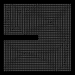
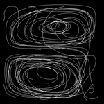
A typical source for vector fields are computational fluid dynamics simulations. In this case, the vector field describes the flow direction of the fluid. A standard technique for visualising them is the use of arrow glyphs representing the local flow direction. Another commonly used method is the visualisation of tangential curves, e.g. path lines for time-dependent vector fields.

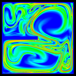
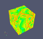
Both approaches have drawbacks in that they visualise only instantaneous local properties (glyphs) and that they are prone to visual clutter (path lines). For time-dependent vector fields, a new approach became popular: the visualisation of Lagrangian coherent structures by using the finite-time Lyapunov (FTLE) exponent. The FTLE is a measure for the separation of particles after a given time. Low FTLE values indicate a low separation and therefore coherent regions in the flow. High FTLE values indicate separation and occur between different coherent regions in the flow. Hence, the FTLE field is separating the flow field in regions of coherent behavior.

Computing the FTLE field is computationally expensive, because an integral curve has to be computed for every element of resulting field. We developed a hierarchical scheme to accelerate this computation. With our method, the computational complexity is reduced from linear to logarithmic. As a result, the computation of a time series of 3D FTLE fields can be done in a few minutes instead of several hours.

2D forward FTLE field of simulated air in a closed room.

3D forward FTLE field of the Arnold-Beltrami-Childress flow.

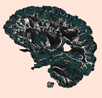
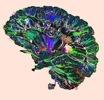
Second-order tensors are used to describe the directional distribution of properties. They are used, e.g. to describe diffusion or mechanical stress. Such data are, for instance, obtained from diffusion tensor magnetic resonance tomography.

One approach to visualise these tensors is the use of special glyphs, similar to arrow glyphs for vectors. However, only local information is directly visible in this case, relations between neighbouring positions are only indirectly recognisable. Another common approach is the display of lines following the major Eigenvector of the tensor, which includes more than local properties in the visualisation. However, this approach is only feasible for a small number of lines. Visualising the complete dataset with this approach results in massive visual clutter.

A possible solution for both problems, visualising not only local properties and avoiding visual clutter, is the extraction and visualisation of structural information from the data. We therefore developed a method to visualise coherent structures in second-order tensor fields.

Visualization of coherent structures in a human brain.

Visualization of nerve tracts in the brain. Coherent regions are consistent with bundles of nerve fibres.